Part 1: Model Compression that Scales in Production
A deep technical dive into LoRA, Knowledge Distillation, Pruning, and Quantization

Deploying a machine learning model is easy. Keeping it performant, efficient, and reliable in the wild is the real challenge. In production, your carefully trained model is exposed to real-world constraints: limited compute, evolving data distributions, and changing business requirements.
This article dives deep into model compression techniques, data distribution shifts, and continual learning strategies, with actionable examples, code snippets, and practical insights for ML engineers.
1. Model Compression: Making Large Models Deployable
Large neural networks achieve state-of-the-art performance, but deploying them directly in production often leads to unacceptable latency, high memory consumption, and excessive inference cost. Model compression techniques reduce the footprint of your model while preserving accuracy.
1.1 LoRA (Low-Rank Adaptation)
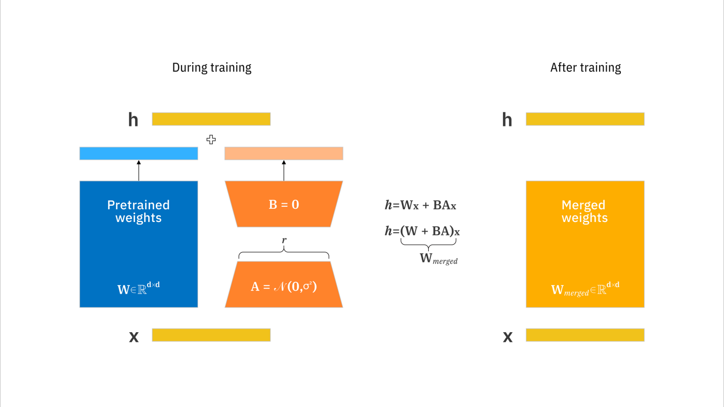
LoRA is a parameter-efficient fine-tuning method for large transformer models. Instead of updating all weights, LoRA introduces low-rank matrices A and B to approximate the weight update:
Here, only A and B are trained during fine-tuning, the original model weights W remain frozen.
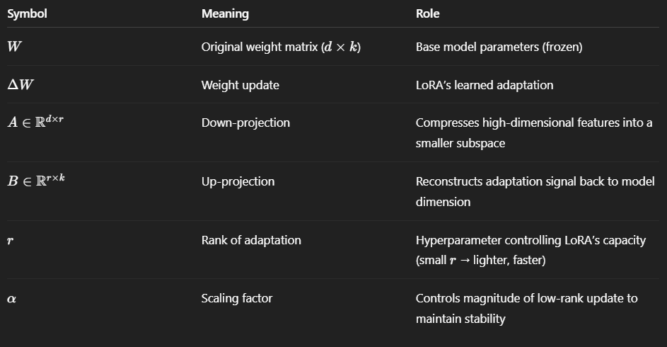
Explanation of terms:
Why Split into Two Matrices (A and B)?
Instead of directly learning a large d×k matrix, LoRA factorizes the update into two smaller matrices A and B:
This drastically reduces trainable parameters from d×k to r(d+k), where r≪min(d,k).
Intuitively:
A: projects input to a compact latent subspace
B: projects back to the original feature space
This low-rank approximation captures the most meaningful directions of change while avoiding the full computational cost.
Role of α (Alpha)
The scaling factor α ensures stable training across different r values.
Prevents updates from being too small (when r is small) or too large.
Decouples adaptation capacity (r) from update strength (α).
Typical choices:
r=4,8,16, and α=8r or 16r
Connection to PEFT (Parameter-Efficient Fine-Tuning)
PEFT is a broader framework that includes several methods to fine-tune large models efficiently without updating all parameters.
LoRA is one of the most popular PEFT techniques.
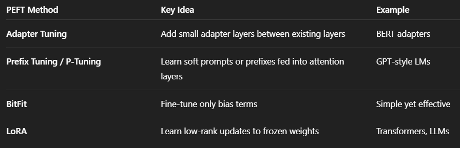
In modern frameworks (like Hugging Face’s PEFT library), LoRA is often implemented on top of large models (e.g., LLaMA, GPT, BERT) by injecting low-rank adapters into attention or feed-forward layers.
This enables:
Memory-efficient training
Fast loading of different fine-tuned adapters
Reusability — one base model, multiple domain-specific LoRA adapters
Why this matters: LoRA enables updating huge models (billions of parameters) on small datasets or limited GPUs. You can adapt models without retraining the entire network.
Real-world example: Updating a deployed language model with company-specific terminology without retraining the entire 70B parameter model.
Code snippet (Hugging Face style LoRA)
from peft import LoraConfig, get_peft_model
from transformers import AutoModelForCausalLM

model = AutoModelForCausalLM.from_pretrained(”gpt-neo-1.3B”)
config = LoraConfig(r=8, lora_alpha=16, target_modules=[”q_proj”, “v_proj”])
lora_model = get_peft_model(model, config)
Explanation of additional terms in code:
r=8: rank of LoRA matrices (small number of parameters to update)lora_alpha=16: scaling factor for the low-rank updateSignificance: larger alpha increases the effective update magnitude
target_modules: layers where LoRA is applied
1.2 Knowledge Distillation
Knowledge Distillation (KD) transfers knowledge from a large teacher model to a smaller student model. The student learns both the original labels and the teacher’s “soft predictions”.

The loss function is:
Explanation of terms:
L_KD: total distillation loss
L_CE(y, y^s): cross-entropy loss between true labels y and student predictions y^s
L_KL: Kullback-Leibler divergence between teacher probabilities p_t and student probabilities p_s
T: temperature parameter
Significance: higher T softens probability distribution, making small differences more noticeable to the student
α: weight balancing true label loss and teacher imitation
Significance: α ≈ 0.5 balances learning from true labels and teacher signals
Why this matters: KD enables smaller, faster models to retain performance of large models, critical for mobile or edge deployment.
Code snippet (PyTorch)
import torch
import torch.nn.functional as F

def distillation_loss(student_logits, teacher_logits, labels, T=2.0, alpha=0.5):
    ce_loss = F.cross_entropy(student_logits, labels)
    kl_loss = F.kl_div(F.log_softmax(student_logits/T, dim=1),
                       F.softmax(teacher_logits/T, dim=1),
                       reduction=’batchmean’) * (T**2)
    return alpha*ce_loss + (1-alpha)*kl_loss
1.3 Pruning
Pruning removes redundant weights or neurons to reduce computation.
Magnitude-based pruning formula:
Explanation of terms:
w_ij: weight of the connection from neuron i to j
θ: pruning threshold; weights smaller than θ are removed
Significance: removing small weights typically has minimal impact on model performance
Intuition: Small-magnitude weights often contribute little to model outputs and can be safely removed, leaving the network functionally similar while reducing computations.
Advanced Pruning Techniques
Structured Pruning
Removes entire neurons, channels, or attention heads.
Hardware-friendly since it reduces matrix dimensions directly.
Example: pruning convolutional filters in CNNs to speed up GPU inference.
Unstructured Pruning
Removes individual weights based on magnitude or importance scores.
Can achieve higher sparsity but may require sparse matrix operations for speedup.
Commonly paired with specialized libraries like NVIDIA’s SparseML or PyTorch sparse modules.
Gradient-Based / Sensitivity Pruning
Uses weight gradients or second-order derivatives (Hessian) to measure sensitivity:
\(\Delta L \approx \frac{1}{2} H_{ii} (\Delta w_i)^2\)Weights with minimal impact on loss (ΔL) are pruned.
Provides more principled pruning than magnitude alone.
Layer-wise or Global Pruning
Layer-wise: prune a fixed fraction of weights per layer
Global: prune weights across all layers based on overall importance
Global pruning often achieves better sparsity-performance trade-offs.
Real-World Example
Recommendation models: structured pruning of fully connected layers can reduce inference latency by 30–40% with <1% accuracy drop.
Transformer models: pruning attention heads and feed-forward neurons allows faster inference while retaining most of the model’s language understanding.
1.4 Quantization
Quantization converts high-precision numbers (like 32-bit floats) into lower-precision numbers (like 8-bit integers) to reduce model size and computation cost.
We generally map a floating-point weight ‘w’ to a lower-bit integer ‘q’ using a linear transformation. We calculate the quantized values using these equations to ensure the integer representation closely approximates the original weights.
Example: FP32 → INT8.
These two equations are designed to linearly map the original floating-point weights to the integer range. The scale factor ‘s’ ensures that the full dynamic range of the weights fits within the target bit-width, while subtracting w_min shifts the range so the smallest weight maps to zero.
This systematic mapping preserves the relative differences between weights, allowing the quantized model to approximate the original model’s behavior with minimal accuracy loss.
Explanation of terms:
w: original weight
w_q: quantized weight
w_min, w_max: minimum and maximum weight values
s: scale factor to map original weights to integer range
b: number of bits (e.g., 8 for INT8)
Why this matters: Reduces memory and inference time without significant accuracy loss, especially on hardware supporting low-precision arithmetic.
Code snippet (PyTorch)
import torch.quantization as tq

model.eval()
quantized_model = tq.quantize_dynamic(model, {torch.nn.Linear}, dtype=torch.qint8)
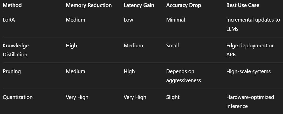
Compression Comparison Table
Techniques like LoRA, knowledge distillation, pruning, and quantization let engineers adapt massive models to limited resources without sacrificing performance. By strategically applying these methods, you can ensure your models stay practical, scalable, and production-ready.